Commonly Used Commands in MATLAB

1. sin(x) >> Computes sine value of x radian.
To plot a sine wave we use the following commands
syntax: t = 0:0.01:1
y = a*sin(w*t); %a = amplitude
plot(t,y)
note: y is a column matrix which contains all the value to plot sine wave

2. cos(x) >> Computes the cosine value of x radian. This is similar to sin(x).

3. plot >> plots a continuous wave.
e.g: plot(t,z) This plots a continuous wave, with t on x axis and z on y axis.
Note: It's important that both the matrix are of same size.

4. subplot >> The figure window is split according to our commands.
e.g: subplot(2,2,1) >> This will divide the figure window into a 2x2 matrix, and the 1st one is accessed now to draw.
Note: plot and stem functions should be used only after subplot function

5. stem >> It is the discrete domain counter part of plot.

6. xlabel('Text') >> This command is usually used after plot and stem function. This command will give a label named 'Text' to x axis of the plot.
e.g: plot(t,y);
xlabel('Time')
ylabel('Amplitude')
title('Sine Wave')

8. ylabel('Text') >> Similar to xlabel.

9. title('Text') >> Gives the title to a plot or subplot.

10. abs(x) >> The command computes the absolute value of x. If x is complex it returns the magnitude.

11. angle(x) >> this command computes the phase angle of x in rad.

12. ones(p,q) >> generates a p x q matrix of ones.

13. zeros(p,q) >> generates a p x q matrix of zeros.

14. mod(m,N) >> Computes m mod N.

15. rem(n,M) >> returns the reminder after dividing n by M.

16. log10(x) >> Computes the base 10 logarithm of elements of x.

17. axis([xmin xmax ymin ymax]) >> Sets scaling for x and y axes for the current plot.



querrymail@gmail.com

Butteworth Filter Design

As the first step, the various commonly used functions are discussed briefly. After that programs are given.

buttord

This functiion returns the order and natural cut-off frequency of the butterworth filter. Its input are passband freq, stopband freq, passband attenuation and stoopband attenuation. The freq must be normalised.

[N,Wn] = buttord(omp,oms,alphap,alphas);
N is the order, Wn is the cut-off.

butter
This is used to get the system function. The numeratoe and denomiantor values are obtained in an array.

[B,A] = butter(N,Wn);


abs

This gives the absolute value of a complex quantity.
m = abs(X);

angle

This will return the phase angle associated with a complex quantity.
an = angle(X);

subplot

This function is very commonly used one. It working can be described through an example.
subplot(3,1,1) means the entire window is divided into a 3X1 matrix and the active portion at the present time is the first one.

plot

It performs the plotting function of qnty. vs other.
plot(Y,X) plots Y as function of X. ie, Y on y axis and X on xaxis.

grid

It will draw grid lines to the plot.

Lowpass Filter

%To design a Butterworth Lowpass Filter
%specifications
clear all
alphap = 4; %Passband Attenuation
alphas = 30; %Stopband attenuation
fp = 400; %Passband frequency in Hz
fs = 800; %Stopband frequency in Hz
F = 2000; %Sampling Frequency in Hz
omp = 2*fp/F;
oms = 2*fs/F;

%To find cut-off frequency and order of filter
[N,Wn] = buttord(omp,oms,alphap,alphas); %N is the order of filter, and Wn is its natural frequency

%System function of filter
[B,A] = butter(N,Wn);
w = 0:0.01:pi;
[h,om] = freqz(B,A,w,'whole'); %h is the complex value of filter corres. to freq w
m = abs(h); %Absolute value of h
an = angle(h); %Angle of h

subplot(2,1,1);
plot(om/pi,20*log(m));
grid;
xlabel('Normalised frequency');
ylabel('Gain in dB');

subplot(2,1,2);
plot(om/pi,an);
grid;
xlabel('Normalised frequency');
ylabel('Phase in radian');


Bandpass Filter

%To design a Butterworth Bandpass Filter
%Specifications
clear all
alphap = 2; %Passband Attenuation
alphas = 20; %Stopband Attenuation
wp = [0.2*pi,0.4*pi]; %Passband Frequency
ws = [0.1*pi,0.5*pi];

%to find cut-off frq and order
[n,wn] = buttord(wp/pi,ws/pi,alphap,alphas);

%System function
[b,a] = butter(n,wn);
w = 0:0.01:pi;
[h,ph] = freqz(b,a,w);
m = 20*log10(abs(h));
an = angle(h);

subplot(2,1,1);
plot(ph/pi,m);
grid;
ylabel('Gain in dB');
xlabel('Normalised Frequency');

subplot(2,1,2);
plot(ph/pi,an);
grid;
ylabel('Phase in radian');
xlabel('Normalised frequency');


Bandreject Filter

%To design a Butterworth bandreject filter
%Specification
clear all
alphap = 2; %Passband attenuation
alphas = 20; %Stopband attenuation
ws = [0.2*pi,0.4*pi]; %Stopband frequency in rad/s
wp = [0.1*pi,0.5*pi]; %Passband frequency in rad/s
%To find cut-off frequency and order
[n,wn] = buttord(wp/pi,ws/pi,alphap,alphas);
%To find system function
[b,a] = butter(n,wn,'stop'); %[b,a] is [numerator,denominator]
w = 0:0.01:pi;
[h,ph] = freqz(b,a,w);
m = 20*log(abs(h));
an = angle(h);
%Plotting
subplot(2,1,1);
plot(ph/pi,m,'r');
grid;
ylabel('Gain in dB');
xlabel('Normalised frequency');
subplot(2,1,2);
plot(ph/pi,an,'b');
grid;
ylabel('Phase in rad');
xlabel('Normalised frequency');



Highpass Filter

%To design a Highpass Butterworth filter
%Specification
clear all
alphap = 4; %Passband attenuation
alphas = 30; %Stopband attenuation
fs = 400; %Stopband frequency in Hz
fp = 800; %Passband frequency
F = 2000;
omp = 2*fp/F; %Normalised
oms = 2*fs/F; %Normalised
%To find cut-off and order
[n,wn] = buttord(omp,oms,alphap,alphas)
%System function
[b,a] = butter(n,wn,'high');
w = 0:0.01:pi;
[h,om] = freqz(b,a,w);
m = 20*log(abs(h));
an = angle(h);
%Plotting
subplot(2,1,1);
plot(om/pi,m);
grid;
ylabel('Gain in db');
xlabel('Normalised frequency');
subplot(2,1,2);
plot(om/pi,an);
grid;
ylabel('Phase in rad');
xlabel('Normalised frequency');



querrymail@gmail.com

MATLAB Overview

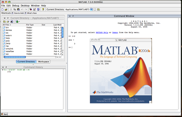Matlab is a commercial "Matrix Laboratory" package which operates as an interactive programming environment. Matlab is well adapted to numerical experiments since the underlying algorithms for Matlab's builtin functions and supplied m-files are based on the standard libraries LINPACK and EISPACK.
Matlab program and script files always have filenames ending with ".m". The programming language is straightforward since almost every data object is assumed to be an array. Graphical output is available to supplement numerical results.
Online help is available from the Matlab prompt (a double arrow), both generally (listing all available commands):

>> help
[a long list of help topics follows]
and for specific commands:

>> help fft
[a help message on the fft function follows].

How to quit Matlab?

Leave a Matlab session by typing

quit
or by typing

exit
to the Matlab prompt.

Building Matrices

Matlab has many types of matrices which are built into the system.

A 7 by 7 matrix with random entries is produced by typing

rand(7)

To generate random matrices of other sizes :

rand(4,6)

To get Hilbert Matrix

hilb(5)

A 5 by 5 magic square :

magic(5)
Tip: A magic square is a square matrix which has equal sums along all its rows and columns. Matrix multiplication is used to check this property.

Some standard matrices from linear algebra :

eye(6)
zeros(4,7)
ones(5)

Single row matrix(the entered values are shown):

[1 2 3 5 7 9]

A 3x3 matrix:
[1, 2, 3; 4, 5, 6; 7, 8, 9]

Variables

Some Built-in variables : pi,eps,ans

To know the active variables at any time use who:

who

help who

To remove a variable

clear x

x

who



querrymail@gmail.com

BASIC MATLAB PROGRAMS

WAVEFORM GENERATIONS

1. SINUSOIDAL SIGNALS
%program starts.
a=input("Enter amplitude=");
f=input("Enter frequency=");
t=0:0.01:1
y=a*sin(2*pi*f*t);
plot(t,y) %gives analog plot
xlabel("TIME");
ylabel("AMPLITUDE");
title("SINE WAVE");

2. RAMP SIGNAL

%program starts
n=input("Enter the Length of Sequence=");
t=0:1:n
stem(t,t) %gives discrete plot
xlabel("TIME");
ylabel(AMPLITUDE");
titile("DISCRETE RAMP SIGNAL");

3. SINE & COSINE WAVEFORMS IN A SINGLE PLOT

%program starts.
a=input("Enter amplitude=");
f=input("Enter frequency=");
t=0:0.01:1
y=a*sin(2*pi*f*t);
z=a*cos(2*pi*f*t);
plot(t,y,z) %gives analog plot of sin & cos in single graph
xlabel("TIME");
ylabel("AMPLITUDE");
title("SINE AND COSINE WAVE");

4. SQUARE WAVE

a=input("Enter amplitude=");
f=input("Enter frequency=");
t=0:0.01:1
y=a*square(2*pi*f*t);
plot(t,y) %gives analog plot
xlabel("TIME");
ylabel("AMPLITUDE");
title("SQUARE WAVE");

5. UNIT STEP AND UNIT IMPULSE FUNCTION AS SUBPLOTS

%subplot means different functions are shown on a single window
%as different graphs.
%subplot(x1,x2,p) means the window is divided into an x1 X x2 matrix.
%and the function is plotted on pth subplot

a=input("Enter amplitude=");
t=-2:1:a-1
y=[zeros(1,2),ones(1,a)];
z=[zer0s(1,20,ones(1,1),zeros(1,a)];
subplot(2,1,1)
stem(t,y)
xlabel("TIME");
ylabel("AMPLITUDE");
title("UNIT STEP SEQUENCE");
subplot(2,1,2)
stem(t,z)
xlabel("TIME");
ylabel("AMPLITUDE");
title("UNIT IMPLUSE SEQUENCE");



querrymail@gmail.com