Reversing a String

;8086 program to reverse the entered string

data segment
msg1 db "Enter the string: $"
msg2 db 0ah,0dh,"Reversed string is: $"
ent db 0dh,0ah,"$"
str1 db 100 dup(?)
rev db 100 dup(?)
data ends

print macro msg
lea dx,msg
mov ah,09h
int 21h
endm

read macro
mov ah,01h
int 21h
endm

code segment
start:
mov ax,data
mov ds,ax

mov bx,0000h
lea si,str1
print msg1

L1:
read
mov [si],al
inc bx
inc si
cmp al,0dh
jnz L1


dec si
mov cx,bx
lea di,rev

L2:
mov al,[si]
mov [di],al
inc di

dec si
dec cx
jnz L2

print msg2
add si,bx

mov cx,bx
print ent

L3:
mov dl,[si]
mov ah,02h
int 21h
dec si
dec cx
jnz L3


en:

mov ah,4ch
int 21h
code ends
end start

;Program ends Here

querrymail@gmail.com

Getting an Input from Keyboard and Displaying it

;8086 program to get an Input from Keyboard and Displaying it

data segment
msg db "Enter a character: $"
msg1 db 0dh,0ah, "The Entered character is:$"
data ends
print macro msg
lea dx,msg
mov ah,09h
int 21h
endm
read macro
mov ah,01h
int 21h
endm
display macro
mov ah,02h
int 21h
endm
code segment
start:
mov ax,data
mov ds,ax
print msg
read
mov bl,al
print msg1
mov dl,bl
display
mov ah,4ch
int 21h
code ends
end start

;Program Ends Here

querrymail@gmail.com

Display a Message on DOS Prompt

This 8086 program compiled in MASM compiler displays the word welcome on the screen.

;Program Starts Here

msg1 db "hello$"
data ends
code segment
start:
mov ax,data
mov ds,ax
lea dx,msg1
mov ah,09h
int 21h
mov ah,4ch
int 21h
code ends
end start

;Program Ends Here

data segment

querrymail@gmail.com

Electronic Rain Guage

CIRCUIT DESCRIPTION

Electronic rain gauge can measure the rainfall of a day. The circuit consists of a sensing section, Micro controller section and a display section.

Sensing section

The sensing section includes a uniform cylindrical collector, 9V dc battery, the voltage regulator IC 7805 and the NOT gate IC 4069N. The 9V DC battery and 7805 regulator provide VCC supply of +5V. The connecting wires are used as the sensors. We use 7 wires and are cut 1cm apart and the longest wire is connected from VCC. fixed at the bottom base of the collector by drilling. Rest of six sensing wires are also fixed 1 cm apart from the base by drilling for recording 5cm and above rainfall and these wires are connected to corresponding inputs of the 6 NOT gates.

If there is no rain, collector is empty and no high signal is at the input of NOT gates. When the water level of collector reaches 1 cm, then the VCC wire at the base and first sensing wire fixed at 1 cm of collector is shorted. Now a high signal (+5V) reaches the input of the first NOT gate. Thus the output of the gate becomes low (zero) Similarly when water level at 2 cm of collector, second sensing wire also got connection with the VCC. Now out put of corresponding not gate also come low. Since the capacity of our rain gauge is 6 cm when the water reaches the top of the collector all the sensing wires are connected with VCC. Now all the inputs of NOT gates are feed from VCC. , out put will become low.

Micro controller section

In the rain gauge we use PIC 16F877A micro controller. It is clocked by crystal oscillator for getting maximum operating Frequency of 20 MHz. It also get supply from the same +5V VCC. Here D port is assigned as input port and C as the out put port.

The output from the NOT gates are connected to the input port lines. ie. out put of the 1st Not gate is connected to Port line D0 , Second gate to D1, like wise 6th gate to D5. All the D ports are set initially. When no rain, there is no change of out put from the NOT gate and initial condition of the D port remains as such; ie. all are set.

When water level rises to 1 cm the out put of first NOT gate become low and low signal reaches the port D0 and it is reset. (ie. Become zero). Similarly when water level at 2 cm the out put of second NOT also become low and gradually port D1, is reset. This will continue up to the capacity of the gauge. Ie. When water reaches top level then out put of all NOT gates will be zero and, the ports D0,D1,D2,D3,D4,D5 are set.

Display Section

Display section include 16 x 2 LCD. The LCD contrast is adjusted by using a 10K port. Here LCD is interfaced with PIC 16F877A. In spite of assigning Port C as out put the port A is also assigned as output by resetting it. Now from Port C connections are made to LCD for data part and from port A connections are made for control part ie. Port A2 is connected to the 4th Pin (RS pin) of LCD to Select command or data register, and A5 is connected to 6th pin (E Pin) to disable or enable LCD. Port C0 to C4 are connected to LCD for display data part.


PIC 16F877A and LCD are interfaced and programmed such that, LCD should display the required information about the rain fall. LCD is 16 x 2, the first line of LCD is made permanent display as “RAIN GAUGE”, using program. Second line is for display information about rain fall. The PIC is [ programmed such a way that, when port D is in unchanged stage ie. all are set then LCD will display LOW/NO RAIN. When port D0 become Low (Zero) then “1 cm Rain” will be displayed on LCD. Similarly when D1, is reset, then LCD will display “2cm Rain”. Likewise when water level reaches top of the collector, all D0.,D1,D2,D3,D4 and D5 Ports are reset, then it is programmed such that “Heavy rain” will be the display.

Thus sensor section, PIC section and display section, perform their work synchronically to display the accurate rainfall and do its duty as a “Electronic Rain Gauge”.

Program

;Program Starts Here

#include <16F877a.h>
#include
#include
main()
{ char no[]="Low/No ",hi[]="Heavy ",cm[]=" cm ",clr[]=" ";
char po[]="Rain Guage",ra[]="Rain";
int val,set,i;
trisd=0xff;
lcdinit();
///misc
go(0);
printc(po);
delay_ms(300);
ra2=0;
for(i=0;i<5;i++)
{
portc=0x1c;
ok();
delay_ms(500);
}
for(i=0;i<3;i++)
{
portc=0x18;
ok();
delay_ms(500);
}
for(i=0;i<4;i++)
{

portc=0x8;
ok();
delay_ms(500);
portc=0x0C;
ok();
delay_ms(1000);
}
portc=1;
ok();
ra2=1;
///end
// position 0, 1... first row, 64,65,....Second row
go(3);
printc(po);

while(1)

{


// delay_ms(1000);
val=portd;

switch(val)
{
case 0xfe:
printc(clr);
go(67);
printh(1); //1
printc(cm);
printc(ra);
break;
case 0xfc:
printc(clr);
go(67);
printh(2);
printc(cm);
printc(ra); //2
break;

case 0xf8:
printc(clr);
go(67);
printh(3);
printc(cm);
printc(ra); //3
break;
case 0xf0:
printc(clr);
go(67);
printh(4);
printc(cm);
printc(ra); //4
break;
case 0xe0:
printc(clr);
go(67);
printh(5);
printc(cm); //5
printc(ra);
break;
case 0xc0:
printc(clr);
go(67);
printh(6);
printc(cm); //6
printc(ra);
break;
case 0x80:
printc(clr);
go(67);
printc(hi); //7
printc(ra);
break;

default:
printc(clr);
go(67);
printc(no); //No
printc(ra);
}
}
}

;Programmed in C
;Program Ends Here

Source: We got this idea from EFY Magazine.

PC Based Oscilloscope Using Matlab

Visit this link:

http://www.mathworks.com/matlabcentral/fileexchange/13165

You can download a .zip file. Unpack and use the oscilloscope.
But it uses your PC's sound card as interface. And also its frequency range is limited to 20Hz-20kHz. Higher frequencies can damage your sound card.

Octave: Open Source Alternative for Scilab

Octave, a freely redistributable software, is used for numerical computation with an interactive environment. Students pick up the basics quickly, comfortably using it within just a few hours. High-level language application intended primarily for numerical computations and other numerical experiments using a language that is compatible with Matlab. It is customizable with user-defined functions written in Octave's language or C++, C, Fortran or others.


For more:

http://www.osalt.com/octave

querrymail@gmail.com

Built-in Functions in Scilab

Most built in functions are identical in Matlab and Scilab. Some of them have a slightly different syntax. Here is a brief, partial list of commands with significant different syntax.

Matlab Scilab "equivalent"

all and

any or

balance balanc

clock unix('date')

computer unix_g('machine')

cputime timer

delete unix('rm file')

dir unix_g('ls')

echo mode

eig spec or bdiag

eval evstr

exist exists + type

fclose file('close')

feof

ferror

feval evstr and strcat

filter rtitr

finite (x < %inf)
fopen file('open') fread read fseek file ftell fwrite writeb global home isglobal isinf(a) a == %inf isnan(a) a ~= a isstr(a) type(a) == 10 keyboard pause + resume lasterr lookfor apropos more lines pack stacksize pause halt qz gspec+gschur randn rand rem modulo setstr code2str strcmp(a,b) a == b uicontrol uimenu getvalue unix unix_g version which whereis nargin [nargout,nargin]=argn(0) nargout

You will get a detailed tutorial on Scilab from: http://www-irma.u-strasbg.fr/~sonnen/SCILAB_HELP/frame.html

querrymail@gmail.com

Scilab: An Alternative to MATLAB

What is Scilab?

Developed at INRIA, SCILAB has been developed for system control and signal processing applications. It is freely distributed in source code format. The following points will explain the features of SCILAB. It is a similar to MATLAB, which is not freely distributed. It has many features similar to MATLAB.
Scilab is made of three distinct parts:

• An interpreter
• Libraries of functions (Scilab procedures)
• Libraries of Fortran and C routines.

SCILAB has an inherent ability to handle matrices (basic matrix manipulation, concatenation, transpose, inverse etc.,)

Scilab has an open programming environment where the creation of functions and libraries of functions is completely in the hands of the user.
Scilab has an open programming environment where the creation of functions and libraries of functions is completely in the hands of the user

Download Scilab:
http://www.scilab.org/download/index_download.php?page=release#windows

What are the main differences between Scilab and MATLAB?
Functions

Functions in Scilab are NOT Matlab m-files but variables. One or several functions can be defined in a single file (say myfile.sci). The name of of the file is not necessarily related to the the name of the functions. The name of the function(s) is given by

function [y]=fct1(x)
...
function [y]=fct2(x)
...

The function(s) are not automatically loaded into Scilab. Usually you have to execute the command getf("myfile.sci") before using it.

Functions can also be defined on-line (or inside functions) by the command deff.

To execute a script file you must use exec("filename") in Scilab and in Matlab you just need to type the name of the file.
Comment lines

Scilab comments begins with: //

Matlab comments begins with: %

Variables

Predefined variables usually have the % prefix in Scilab (%i, %inf, ...). They are write protected.

Strings

Strings are considered as 1 by 1 matrices of strings in Scilab. Each entry of a string matrix has its own length.

Boolean variables

Boolean variables are %T, %F in Scilab and 0, 1 in Matlab. Indexing with boolean variables may not produce same result. Example x=[1,2];x([1,1]) [which is NOT x([%T,%T])] returns [1,1] in Scilab and [1,2] in Matlab. Also if x is a matrix x(1:n,1)=[] or x(:)=[] is not valid in Matlab.

Polynomials

Polynomials and polynomial matrices are defined by the function poly in Scilab (built-in variables). They are considered as vectors of coefficients in Matlab.

Empty matrices

[ ]+1 returns 1 in Scilab and [ ] in Matlab.

Plotting

Except for the simple plot and mesh (plot3d) functions, Scilab and Matlab are not compatible.

Scicos

Scicos (Scilab) and Simulink (Matlab) are not compatible.

querrymail@gmail.com

IR Tracking Robot

I got idea from EFY magazine and implemented along with my friends. It works well.

AMV: A Monostable Multivibrator

The robot described here senses a 38 kHz IR radiations and moves towards that direction. The system consists of three sections viz., sensor, controller and driver. The sensing section detects the 38 kHz IR radiation. The controller section processes the information from the sensor and provides the input to the driver section which has stepper motors for driving the robot.

The output of the sensors is fed to the monostable multivibrator which serves as the input to the microcontroller. Depending on the input sequence obtained the microcontroller performs sequential operation and gives out its decisions, which is a sequence of bits to drive stepper motors.

Since the microcontroller output is not sufficient to drive the stepper motor, a high voltage, high current Darlington array has been used to drive the motors. In the process of reaching the target, if an obstacle is encountered, the robot changes its path and again starts tracking the incoming IR radiation.

Robot Sensing Section


Robot Driving Section







Program

;Program Starts Here
$MOD51
ORG 0000H
CLR A
MOV P1, A
MOV P2, A
MOV P3, #0FFH
MOV R1, #11H
MOV R2, #11H
BACK: MOV C, P3.2
JB P3.0, NEXT
CPL C
NEXT: ANL C, P3.1
JC STRAIGHT
MOV C, P3.1
ANL C, P3.2
CPL C
ANL C, P3.0
JC LEFT
MOV C, P3.2
ORL C, /P3.1
ANL C, /P3.0
JC RIGHT
LJMP BACK
LEFT: MOV R3, #04H
FIRST: MOV A, R2
MOV P2, A
ACALL DELAY
RL A
MOV R2, A
DJNZ R3, FIRST
LJMP BACK
RIGHT: MOV R4, #04H
SECOND: MOV A, R1
MOV P1, A
ACALL DELAY
RR A
MOV R1, A
DJNZ R4, SECOND
LJMP BACK
STRAIGHT: MOV R3, #04H
THIRD: MOV A, R1
MOV P1, A
RR A
MOV R1, A
MOV A, R2
MOV P2, A
RL A
MOV R2, A
ACALL DELAY
DJNZ R3, THIRD
LJMP BACK
DELAY: MOV R6, #64
H1: MOV R7, #255
H2: DJNZ R7, H2
DJNZ R6, H1
RET
END

;Program Ends Here

Source: EFY Magazine

querrymail@gamail.com

Analyzing a .wav file

In the previous article we found how to create a simple audio music file. Here, we are going to analyze it, i.e., to find out the fundamental frequency and other parameters. The code given below plots the .wav file and it power spectrum.

%Code Starts here

[y, Fs] = wavread(file); % y is sound data, Fs is sample frequency.
t = (1:length(y))/Fs; % time

ind = find(t>0.1 & t<0.12); % set time duration for waveform plot
figure; subplot(1,2,1)
plot(t(ind),y(ind))
axis tight
title(['Waveform of ' file])

N = 2^12; % number of points to analyze
c = fft(y(1:N))/N; % compute fft of sound data
p = 2*abs( c(2:N/2)); % compute power at each frequency
f = (1:N/2-1)*Fs/N; % frequency corresponding to p

subplot(1,2,2)
semilogy(f,p)
axis([0 4000 10^-4 1])
title(['Power Spectrum of ' file])

%Code ends here

querrymail@gmail.com

Generate Music using MATLAB

This is an interesting, but simple experiment which has many utility. The following code can genrate a .wav file to play a sound of required frequency.

Before proceeding you should set the following:
filename---> give a name to your fantastic music file (say 'mymusic.wav')
f-----------> fundamental frequency (say f=256) in Hz.
d----------> time duration (say t =5) in seconds.
p----------> it is vector of amplitudes of length n. (say it values be [1 0.8 0.1 0.04]

%Code starts here

Fs=22050; nbits=8; % frequency and bit rate of wav file
t = linspace(1/Fs, d, d*Fs); % time
y = zeros(1,Fs*d); % initialize sound data
for n=1:length(p);
y = y + p(n)*cos(2*pi*n*f*t); % sythesize waveform
end
y = .5*y/max(y); % normalize. Coefficent controls volume.
wavwrite( y, Fs, nbits, filename)

%Code ends here

querrymail@gmail.com

Addition of two numbers

data segment
msg1 db "Enter the first 2 digit number: $"
msg2 db 0dh,0ah,"Enter the second 2 digit number: $"
msg3 db 0dh,0ah,"Sum = $"
data ends

print macro msg
lea dx,msg
mov ah,09h
int 21h
endm

read macro
mov al,01h
int 21h
endm

display macro num
mov dl,num
mov al,02h
int 21h
endm

code segment
start:mov ax,data
mov ds,ax

print msg1
read
mov bh,al
read
mov bl,al
print msg2
read
mov ch,al
read
mov cl,al

mov ax,bx
add al,cl
aaa
mov bl,al
mov al,ah
add al,ch
aaa
mov cx,ax

add cl,30h
add ch,30h
add bl,30h
print msg3
display ch
display cl
display bl

code ends
end start

querrymail@gmail.com

Palindrome

This is a program in 8086 ASM to check the given string is palindrome or not.
The program is compiled in MASM compiler.

data segment
msg1 db "Enter the string: $"
msg2 db 0ah,0dh,"Reversed string is: $"
msg3 db 0dh,0ah,"Not palindrome...........$"
msg4 db 0dh,0ah," palindrome...........$"
ent db 0dh,0ah,"$"
str1 db 100 dup(?)
rev db 100 dup(?)
data ends

print macro msg
lea dx,msg
mov ah,09h
int 21h
endm

read macro
mov ah,01h
int 21h
endm

code segment
start:
mov ax,data
mov ds,ax
mov bx,0000h
lea si,str1
print msg1

L1:
read
mov [si],al
inc bx
inc si
cmp al,0dh
jnz L1


dec si
mov cx,bx
lea di,rev

L2:
mov al,[si]
mov [di],al
inc di

dec si
dec cx
jnz L2

print msg2
add si,bx

mov cx,bx
print ent

L3:
mov al,[si]
mov dl,al
mov ah,02h
int 21h
dec si
dec cx
jnz L3

sub di,bx
mov cx,bx

L4:
dec cx
jz p
inc si
inc di
mov al,[si]
cmp al,[di]
jz L4
print msg3 ;not paliandrome
jmp en

p:
print msg4 ;paliendrome
en:
mov ah,4ch
int 21h
code ends
end start

ret


querrymail@gmail.com

Multiplication

This 8086 program multiplies two numbers.

data segment
msg1 db "Enter the first number: $"
msg2 db 0dh,0ah, "Enter the second number: $"
msg3 db 0dh,0ah, "Product= $"
data ends

print macro msg
lea dx,msg
mov ah,09h
int 21h
endm

read macro
mov ah,01h
int 21h
endm

display macro num
mov dl,num
mov ah,02h
int 21h
endm

code segment
start:mov ax,data
mov ds,ax
print msg1 ;read 1st number
read
mov bh,al
read
mov bl,al
print msg2 ;read 2nd number
read
mov ch,al
read
mov cl,al
sub bx,3030h
sub cx,3030h
mov dl,bh
rol dl,4
add bl,dl
mov dl,ch
rol dl,4
add cl,dl
and bx,00ffh
and cx,00ffh
mov ax,bx ;multipilication starts
mul cx
mov bx,dx
mov cx,ax
add bx,3030h
add cx,3030h
print msg3
display bh
display bl
display ch
display cl
mov ah,4ch
int 21h
code ends
end start


querrymail@gmail.com

Square Root

;8086 program that computes the square root of a perfect square number

data segment
msg1 db "Enter the number:$"
msg2 db 0ah,0dh, "The entered number is not a perfect square$"
msg3 db 0ah,0dh, "Square root is:$"
data ends

print macro msg
lea dx,msg
mov ah,09h
int 21h
endm

read macro
mov ah,01h
int 21h
sub al,30h
mov bh,0ah
mul bh
mov bl,al
mov ah,01h
int 21h
sub al,30h
add bl,al
endm

disp macro reg
mov dl,reg
mov ah,09
int 21h
endm

code segment
start:
mov ax,data
mov ds,ax

print msg1
read

mov cl,00h
mov ch,01h
l3:
sub bl,ch
jc l2
jz l1
;aas
inc cl
inc ch
inc ch
jmp l3
l1:
inc cl
print msg3
add cl,30h
mov dl,cl
mov ah,02h
int 21h
jmp k
l2:
print msg2
k:
mov ah,4ch
int 21h
code ends
end start

;Program Ends Here

querrymail@gmail.com

JPEG: Joint Photographic Experts Group

In the earlier articles, I described about MPEG and its different versions that are commonly used. MPEG is for the compression of Audio-Video data. But the standard used for the compression of photographic images is JPEG. This article gives you a brief idea about JPEG.

The JPEG group was approved in 1994 as ISO-10918-1.

MPEG 7: Multimedia Content Description Interface

MPEG 7 is formally known as Multimedia Content Description Interface. MPEG 7 is not aimed at a single application. The elements that MPEG 7 standardizes supports broad range of applications.It is a standard for describing the multimedia content data that supports some degree of interpretation of the information meaning, which can be passed onto, or accessed by, a device or a computer code.

The MPEG-7 Standard consists of the following parts:

1. Systems – the tools needed to prepare MPEG-7 descriptions for efficient transport and storage and the terminal architecture.

2. Description Definition Language - the language for defining the syntax of the MPEG-7 Description Tools and for defining new Description Schemes.

3. Visual – the Description Tools dealing with (only) Visual descriptions.

4. Audio – the Description Tools dealing with (only) Audio descriptions.

5. Multimedia Description Schemes - the Description Tools dealing with generic features and multimedia descriptions.

6. Reference Software - a software implementation of relevant parts of the MPEG-7 Standard with normative status.

7. Conformance Testing - guidelines and procedures for testing conformance of MPEG-7 implementations

8. Extraction and use of descriptions – informative material about the extraction and use of some of the Description Tools.

9. Profiles and levels - provides guidelines and standard profiles.

10. Schema Definition - specifies the schema using the Description Definition Language



querrymail@gmail.com

A Peep into MPEG 4

MPEG 4 is audio-video compression standard similar to MPEG 1 and MPEG 2 adapting all the features of MPEG 1 and 2 along new features such as (extended) VRML support for 3D rendering, object-oriented composite files (including audio, video and VRML objects), support for externally-specified Digital Rights Management and various types of interactivity. Its formal designation is ISO/IEC 14496.

MPEG 4 has been proven to be successful in three fields:

• Digital television
• Interactive graphics applications
  
• Interactive multimedia

MPEG 4 consists of several parts, which are described below:

Part 1: System- Describes synchronisation and multiplexing of Audio and video.

Part 2: Visual- Visual data compression.

Part 3: Audio- for perpectual coding of audio signals.

Part 4: Conformance- Describe procedures for testing other parts.

Part 5: Reference Software- For demonstrating and clarifying other parts of the standard.
Part6: Delivery Multimedia Integration framework

Part 7: Optimized Reference Software

Part 8: Carriage on IP networks

Part 9: Reference Hardware
Part 10: Advanced Video Coding (AVC)

Part 11: Scene description and Application engine("BIFS")

Part 12: ISO Base Media File Format- File format for storing media content

Part 13: Intellectual Property Management and Protection (IPMP) Extensions.

Part 14: MPEG-4 File Format
Part 15: AVC File Format
Part 16: Animation Framework eXtension (AFX).
Part 17: Timed Text subtitle format.
Part 18: Font Compression and Streaming.
Part 19: Synthesized Texture Stream.
Part 20: Lightweight Application Scene Representation (LASeR).
Part 21: MPEG-J Graphical Framework eXtension (GFX)

Part 22: Open Font Format Specification (OFFS) based on OpenType

Part 23: Symbolic Music Representation (SMR)


querrymail@gmail.com

About MPEG 2

MPEG 2 is another video standard developed by MPEG Group, but it is not a successor of MPEG1. Both MPEG 1 and MPEG 2 have their own functions: MPEG 1 is for low band width purposes and MPEG 2 for high bandwidth/broadband purposes. The international standard number of MPEG 2 is ISO 13818.

MPEG 2 is commonly used in Digital TVs, DVD Videos, SVCDs etc. Some Blu-ray disks also uses it.

The maximum bit rate available for MPEG-2 streams are 10.08 Mbit/s and the minimum are 300 kbit/s.

Resolutions that video streams can use, are:

720x480 (NTSC, only with MPEG-2)
720x576 (PAL, only with MPEG-2)
704x480 (NTSC, only with MPEG-2)
704x576 (PAL, only with MPEG-2)
352x480 (NTSC, MPEG-2 & MPEG-1)
352x576 (PAL, MPEG-2 & MPEG-1)
352x240 (NTSC, MPEG-2 & MPEG-1)
352x288 (PAL, MPEG-2 & MPEG-1)

The technical title for MPEG 2 is: "Generic coding of moving pictures and associated audio information".

MPEG-2 is a standard currently in 9 parts.

Part 1 of MPEG-2 addresses combining of one or more elementary streams of video and audio, as well as, other data into single or multiple streams which are suitable for storage or transmission. This is specified in two forms: the Program Stream and the Transport Stream. Each is optimized for a different set of applications. A model is given in Figure 1 below.

The Program Stream is similar to MPEG-1 Systems Multiplex. It results from combining one or more Packetised Elementary Streams (PES), which have a common time base, into a single stream. The Program Stream is designed for use in relatively error-free environments and is suitable for applications which may involve software processing. Program stream packets may be of variable and relatively great length.

The Transport Stream combines one or more Packetized Elementary Streams (PES) with one or more independent time bases into a single stream. Elementary streams sharing a common timebase form a program. The Transport Stream is designed for use in environments where errors are likely, such as storage or transmission in lossy or noisy media. Transport stream packets are 188 bytes long.

Part 2 of MPEG-2 builds on the powerful video compression capabilities of the MPEG-1 standard to offer a wide range of coding tools. These have been grouped in profiles to offer different functionalities. Only the combinations marked with an "X" are recognised by the standard.

Part 3 of MPEG-2 is a backwards-compatible multichannel extension of the MPEG-1 Audio standard. The figure below gives the structure of an MPEG-2 Audio block of data showing this property.

Part 4 and 5 of MPEG-2 correspond to part 4 and 5 of MPEG-1.

Part 6 of MPEG-2 - Digital Storage Media Command and Control (DSM-CC) is the specification of a set of protocols which provides the control functions and operations specific to managing MPEG-1 and MPEG-2 bitstreams. These protocols may be used to support applications in both stand-alone and heterogeneous network environments. In the DSM-CC model, a stream is sourced by a Server and delivered to a Client. Both the Server and the Client are considered to be Users of the DSM-CC network. DSM-CC defines a logical entity called the Session and Resource Manager (SRM) which provides a (logically) centralized management of the DSM-CC Sessions and Resources.

Part 7 of MPEG-2 will be the specification of a multichannel audio coding algorithm not constrained to be backwards-compatible with MPEG-1 Audio.

Part 8 of MPEG-2 was originally planned to be coding of video when input samples are 10 bits.

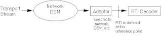
Part 9 of MPEG-2 is the specification of the Real-time Interface (RTI) to Transport Stream decoders which may be utilized for adaptation to all appropriate networks carrying Transport Streams.

Part 10 is the conformance testing part of DSM-CC.


querrymail@gmail.com

More About MPEG 1

The MPEG-1 Audio and video compression format was developed by MPEG group back in 1993. The Official description for it is "Coding of moving pictures and associated audio for digital storage media at up to about 1,5 Mbit/s".

MPEG-1 is the video format that has had some extremely popular spin-offs and sideproducts, most notably MP3 and VideoCD.

MPEG-1's compression method is based on re-using the existing frame material and using psychological and physical limitations of human senses. MPEG-1 video compression method tries to use previous frame's information in order to reduce the amount of
information the current frame requires. Also, the audio encoding uses something that's called psychoacoustics -- basically compression removes the high and low frequencies a normal human ear cannot hear.

Resolutions that video streams can use are:

352x480 (NTSC, MPEG-2 & MPEG-1)
352x576 (PAL, MPEG-2 & MPEG-1)
352x240 (NTSC, MPEG-2 & MPEG-1)
352x288 (PAL, MPEG-2 & MPEG-1)

MPEG-1 standard consists of five parts: named as Part 1 to Part 5.

Part 1 addresses the problem of combining one or more data streams
from the video and audio parts of the MPEG-1 standard with timing
information to form a single stream as in figure.
This is an important fuction because, once combined
into a single stream, the data are in a form well
suited to digital
storage or transmission.


Part 2 specifies a coded representation that can be used for compressing video sequences - both 625-line and 525-lines - to bitrates around 1,5 Mbit/s. Part 2 was developed to operate principally from storage media offering a continuous transfer rate of about 1,5 Mbit/s.

A number of techniques are used to achieve a high compression ratio. The first is to select an appropriate spatial resolution for the signal. The algorithm then uses block-based motion compensation to reduce the temporal redundancy. Motion compensation is used for causal prediction of the current picture from a previous picture, for non-causal prediction of the current picture from a future picture, or for interpolative prediction from past and future pictures. The difference signal, the prediction error, is further compressed using the discrete cosine transform (DCT) to remove spatial correlation and is then quantised. Finally, the motion vectors are combined with the DCT information, and coded using variable length codes.

The figure below illustrates a possible combination of the three
main types of pictures that are used in the standard.

Part 3 specifies a coded representation that can be used for compressing audio sequences - both mono and stereo. The algorithm is illustrated in Figure 3 below. Input audio samples are fed into
the encoder. The mapping creates a filtered and subsampled representation of the input audio stream. A psychoacoustic model creates a set of data to control the quantiser and coding. The
quantiser and coding block creates a set of coding symbols from the mapped input samples. The block 'frame packing' assembles the actual bitstream from the output data of the other blocks, and adds other information (e.g. error correction) if necessary.

Part 4 specifies how tests can be designed to verify whether bit streams and decoders meet the requirements as specified in parts 1, 2 and 3 of the MPEG-1 standard. These tests can be used by:

manufacturers of encoders, and their customers, to verify whether
the encoder produces valid bit streams.

manufacturers of decoders and their customers to verify whether
the decoder meets the requirements specified in parts 1,2
and 3 of the standard for the claimed decoder capabilities.

applications to verify whether the characteristics of a given
bit stream meet the application requirements, for example
whether the size of the coded picture does not exceed the
maximum value allowed for the application.



Part 5, technically not a standard, but a technical report, gives a full software implementation of the first three parts of the MPEG-1 standard.


querrymail@gmail.com

MPEG Compression

MPEG uses an asymmetric compression method. Compression under MPEG is far more complicated than decompression, making MPEG a good choice for applications that need to write data only once, but need to read it many times. An example of such an application is an archiving system.

MPEG uses two types of compression methods to encode video data: interframe and intraframe encoding.

Interframe encoding is based upon both predictive coding and interpolative coding techniques, as described below.

When capturing frames at a rapid rate (typically 30 frames/second for real time video) there will be a lot of identical data contained in any two or more adjacent frames. If a motion compression method is aware of this temporal redundancy, then it need not encode the entire frame of data, as is done via intraframe encoding. Instead, only the differences (deltas) in information between the frames is encoded. This results in greater compression ratios, with far less data needing to be encoded. This type of interframe encoding is called predictive encoding.

A further reduction in data size may be achieved by the use of bi-directional prediction. Differential predictive encoding encodes only the differences between the current frame and the previous frame. Bi-directional prediction encodes the current frame based on the differences between the current, previous, and next frame of the video data. This type of interframe encoding is called motion-compensated interpolative encoding.

To support both interframe and intraframe encoding, an MPEG data stream contains three types of coded frames:

* I-frames (intraframe encoded) * P-frames (predictive encoded) * B-frames (bi-directional encoded)
An I-frame contains a single frame of video data that does not rely on the information in any other frame to be encoded or decoded. Each MPEG data stream starts with an I-frame.

A P-frame is constructed by predicting the difference between the current frame and closest preceding I- or P-frame. A B-frame is constructed from the two closest I- or P-frames. The B-frame must be positioned between these I- or P-frames.

A typical sequence of frames in an MPEG stream might look like this:

IBBPBBPBBPBBIBBPBBPBBPBBI

In theory, the number of B-frames that may occur between any two I- and P-frames is unlimited. In practice, however, there are typically twelve P- and B-frames occurring between each I-frame. One I-frame will occur approximately every 0.4 seconds of video run time.

Remember that the MPEG data is not decoded and displayed in the order that the frames appear within the stream. Because B-frames rely on two reference frames for prediction, both reference frames need to be decoded first from the bit stream, even though the display order may have a B-frame in between the two reference frames.

In the previous example, the I-frame is decoded first. But, before the two B-frames can be decoded, the P-frame must be decoded, and stored in memory with the I-frame. Only then may the two B-frames be decoded from the information found in the decoded I- and P-frames. Assume, in this example, that you are at the start of the MPEG data stream. The first ten frames are stored in the sequence IBBPBBPBBP (0123456789), but are decoded in the sequence:

IPBBPBBPBB (0312645978)

and finally are displayed in the sequence:

IBBPBBPBBP (0123456789)

Once an I-, P-, or B-frame is constructed, it is compressed using a DCT compression method similar to JPEG. Where interframe encoding reduces temporal redundancy (data identical over time), the DCT-encoding reduces spatial redundancy (data correlated within a given space). Both the temporal and the spatial encoding information are stored within the MPEG data stream.

By combining spatial and temporal sub-sampling, the overall bandwidth reduction achieved by MPEG can be considered to be upwards of 200:1. However, with respect to the final input source format, the useful compression ratio tends to be between 16:1 and 40:1. The ratio depends upon what the encoding application deems as "acceptable" image quality (higher quality video results in poorer compression ratios). Beyond these figures, the MPEG method becomes inappropriate for an application.

In practice, the sizes of the frames tend to be 150 Kbits for I-frames, around 50 Kbits for P-frames, and 20 Kbits for B-frames. The video data rate is typically constrained to 1.15 Mbits/second, the standard for DATs and CD-ROMs.

The MPEG standard does not mandate the use of P- and B-frames. Many MPEG encoders avoid the extra overhead of B- and P-frames by encoding I-frames. Each video frame is captured, compressed, and stored in its entirety, in a similar way to Motion JPEG. I-frames are very similar to JPEG-encoded frames. In fact, the JPEG Committee has plans to add MPEG I-frame methods to an enhanced version of JPEG, possibly to be known as JPEG-II.

With no delta comparisons to be made, encoding may be performed quickly; with a little hardware assistance, encoding can occur in real time (30 frames/second). Also, random access of the encoded data stream is very fast because I-frames are not as complex and time-consuming to decode as P- and B-frames. Any reference frame needs to be decoded before it can be used as a reference by another frame.

There are also some disadvantages to this scheme. The compression ratio of an I-frame-only MPEG file will be lower than the same MPEG file using motion compensation. A one-minute file consisting of 1800 frames would be approximately 2.5Mb in size. The same file encoded using B- and P-frames would be considerably smaller, depending upon the content of the video data. Also, this scheme of MPEG encoding might decompress more slowly on applications that allocate an insufficient amount of buffer space to handle a constant stream of I-frame data.


querrymail@gmail.com

MPEG: Moving Picture Expert Group

MPEG stands for Moving Picture Experts Group. It is a family of standards used for coding audio-visual information (e.g., movies, video, music) in a digital compressed format.

The major advantage of MPEG compared to other video and audio coding formats is that MPEG files are much smaller for the same quality. This is because MPEG uses very sophisticated compression techniques.

Moving Picture Experts Group (MPEG) a working group of ISO/IEC in charge of the development of standards for coded representation of digital audio and video. Established in 1988, the group has produced the following compression mechanisms:

MPEG-1: The standard on which such products as Video CD and MP3

MPEG-2: The standard on which such products as Digital Television set top boxes and DVD are based.

MPEG-4: The standard for multimedia for the fixed and mobile web.

MPEG-7: The standard for description and search of audio and visual content.

MPEG-21: The Multimedia Framework.

In addition to these consolidated standards, MPEG has started a number of new standard lines:

MPEG-A: Multimedia application format.

MPEG-B: MPEG systems technologies.

MPEG-C: MPEG video technologies.

MPEG-D: MPEG audio technologies.

MPEG-E: Multimedia Middleware.

MPEG is a working group of ISO, the International Organization for Standardization. Its formal name is ISO/IEC JTC 1/SC 29/WG 11. The title is: Coding of moving pictures and audio.

MPEG held its first meeting in May 1988 in Ottawa, Canada. By late 2005, MPEG has grown to include approximately 350 members per meeting from various industries, universities, and research institutions. Now MPEG has become an inevitable part of modern life.


querrymail@gmail.com

How to make our own functions?

In the previous post I've given a simple example to capture and analyze sound. In it I've used a function daqdocfft which is not a built in one. I got it from Mathworks. Similar to it we can create our own functions for peculiar applications. The function daqdocfft is given below


%================Program====================%

function [f,mag] = daqdocfft(data,Fs,blocksize)
% [F,MAG]=DAQDOCFFT(X,FS,BLOCKSIZE) calculates the FFT of X
% using sampling frequency FS and the SamplesPerTrigger
% provided in BLOCKSIZE

xfft = abs(fft(data));

% Avoid taking the log of 0.
index = find(xfft == 0);
xfft(index) = 1e-17;

mag = 20*log10(xfft);
mag = mag(1:floor(blocksize/2));
f = (0:length(mag)-1)*Fs/blocksize;
f = f(:);

Publish Post

%============Program Ends=======%

function is a built in key word. It should be given in the start to make a function. It is then followed by the return values. Then comes the original name of the new function followed by its arguments. The function name with its arguments is equated to function return_value.
After writing this you can write the code for what the function should do actually.

querrymail@gmail.com

Plotting Real Time Data

In the earlier post, I've described how to communicate with an external MCU from your PC through MATLAB. Now the following section describes how to get real-time data from it and how to plot it on the screen.

The program captures two multiplexed data sent by MCU. It then demultiplex it and plot the values periodcally into the screen.

The received data is stored in a 100x2 matrix, data. It is then plotted.

%==================Pgm Starts=========================%
try
fclose(instrfind)
end

s1 = serial('COM1','BaudRate',2400,'Parity','none','DataBits',8,'StopBits',1);
set(s1,'InputBufferSize',1024);
fopen(s1)
disp('Serial Communication Set Up Complete');

%async mode
s1.Terminator = 13;
s1.Timeout = 10; %Default
s1.ReadAsyncMode = 'continuous';
%readasync(s1);

k = 1;

data = zeros(100,2);

PLOT = 100;

figure(1);

%=======================Plot Set Up and Grab Handles==================%

subplot(2,1,1);
FirstPlot = plot(data(:,1),'g');
hold on;
axis([1 100 0 5]);
title('First Plot');

subplot(2,1,2);
SecondPlot = plot(data(:,2),'b');
hold on;
axis([1 100 0 5]);
title('SecondPlot');

set(FirstPlot,'Erase','xor');
set(SecondPlot,'Erase','xor');


while(1)

data(k,:) = fread(s1,2,'uint8');

%============Updata pLots==================%

set(FirstPlot,'YData',data(:,1));
set(Secondlot,'YData',data(:,2));
drawnow;
%========================================%

k = k+1;

if(k==PLOT)
k=1;
end

end


querrymail@gmail.com

Serial Communication for Real Time Data Capturing

Suppose that we want to send some data to a Microcontroller Unit and get data from it into our PC. MATLAB have wonderful features for implementing this. Here, I attach a program that will send a data to MCU and gets data from MCU. This is accomplished through serial communication. I used COM1 port of my PC.
The data sent by PC is received USART data register of MCU, and it is verified. This is done only for informing the MCU that we want values. On reception of the value MCU begins to send data which is captured by PC.

%==========================PROGRAM============================%

clear all

try
fclose(instrfind) %Close all bogus connections
end

%==First we need to make a serial communication object. Here it is s1.

s1 = serial('COM1','BaudRate',9600,'Parity','none','DataBits',8,'StopBits',1);
set(s1,'InputBufferSize',1024);
fopen(s1);
disp('Communication Set Up Ok')

%async mode
s1.Terminator = 13;
s1.Timeout = 10; %Default
s1.ReadAsyncMode = 'continuous'; %Set communicatio to Asynchronous Mode. You can also
%set it to 'manual' mode.
readasync(s1);


fwrite(s1,'A'); %Informing MCU


data = fread(s1,10,'uint8'); % reads 10 value from microcontroller

plot(data);



querrymail@gmail.com